|
Design
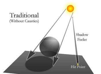 Traditional Ray Tracing Algorithm Traditional Ray Tracing AlgorithmThe problem is that in the real world, the lighting at any point on a surface is not just the result of all lights directly shining on it. Light will bounce off several other objects first before hitting a point on the surface in question. This is compensated for by using ambient lighting in a basic ray tracer. However, one of the reasons people can look at an image and tell that it's been ray traced is because this global lighting is absent (ambient lighting just doesn't cut it). We as humans pick up these small lighting subtleties without even knowing it. 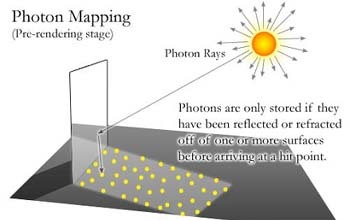
The Photon Map
Implementing the photon mapping algorithm (originally developed by Henrik Wann Jensen in the mid 90's) provides a very practical solution to the global lighting problem.The idea is that before you render your scene, you create a "photon map" by shooting massive amounts of photons from each light source into the scene. These photons will bounce around off the various objects depending on the surface material. If the surface is refractive, then the photon will travel through it. If it is reflective, the photon will bounce off and head into a different direction. The photon will stop when the surface material isn't reflective or refractive. More complicated issues arrive when a material is partially reflective or refractive. For example a material may be 30% reflective. In this case, when a photon comes into contact with it, we store a photon there, but only at 30% of its brightness. Since the photon was not completely absorbed by the material, we create another photon with 70% of the original photon's brightness and have it continue on into the scene via the reflected vector. It is important to note that photons hitting a surface for the first time (directly from the light source) will never be stored there. This is because the regular, direct lighting algorithm used in the ray tracer will take care of it. At each hit point, the local lighting will be computed and then the photon map will be queried to see if any addition indirect light hits the surface at that point. One thing that makes the creation of the photon map a lot easier is that you can adapt your regular ray tracing algorithm to produce the map, which is what I did. Instead of tracing from the eye into the scene, you start at a light source and proceed into the scene looking for intersections. Many of the features in the regular algorithm are directly applicable to this. KD-Tree
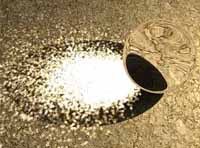 While I was developing the photon map, I first tried it without the KD-Tree structure and instead used a brute-force method to traverse every photon per every hit point. I rendered the image to the right at 800x600 with 386,399 photons in the map. With the brute force method, it took 5.3 hours to render. With the KD-Tree method, it took less than 10 seconds.
Thus, after all the photons are launched and stored into the photon map structure, it is strongly advised that they are restructured into a KD-Tree if you want results sometime this year!
While I was developing the photon map, I first tried it without the KD-Tree structure and instead used a brute-force method to traverse every photon per every hit point. I rendered the image to the right at 800x600 with 386,399 photons in the map. With the brute force method, it took 5.3 hours to render. With the KD-Tree method, it took less than 10 seconds.
Thus, after all the photons are launched and stored into the photon map structure, it is strongly advised that they are restructured into a KD-Tree if you want results sometime this year!The KD-Tree stores the photons very conveniently so that in the final gathering stage (see below) the photons can be searched very fast. This is important since computing the lighting at each hit point will involve "effectively" searching every one of the photons in the entire map to see how close they are to the hit point. The algorithm for creating a balanced KD-Tree is as follows:
Node CreateKDTree (points)
This algorithm effectively divides up the photons at every iteration instead of searching them one by one. The time it takes
to locate a photon in a KD-Tree is, in the worst case, O(log N) where N is the number of photons in the tree. When creating the
KD-Tree, I used Quick Sort to find the median points, which drastically improved the speed.
{ create a 3d cube surrounding all points select the dimension in which the cube is largest find the median of the points according to selected dimension set A = all points below median set B = all points above median this node = median point this node.left = CreateKDTree (set A) this node.right = CreateKDTree (set B) return this node } Gathering Stage
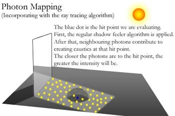 During the final rendering stage, lighting is computed at each hit point. Local direct lighting is first computed, but then the photon map is queried to see if any photons are hanging around to contribute additional lighting. I did this by querying the KD-Tree (photon map) to see what photons are in the specified range. All these photons are gathered together and, depending on how close they are to the hit point and their intensities, they will contribute light. Photons that are closer to the hit point naturally contribute the most. During the final rendering stage, lighting is computed at each hit point. Local direct lighting is first computed, but then the photon map is queried to see if any photons are hanging around to contribute additional lighting. I did this by querying the KD-Tree (photon map) to see what photons are in the specified range. All these photons are gathered together and, depending on how close they are to the hit point and their intensities, they will contribute light. Photons that are closer to the hit point naturally contribute the most. |